< Previous lesson | Overview | Next lesson >
=VLOOKUP()
How to look up values in a grid
=VLOOKUP() is certainly one of the most powerful formulas in Calc. Simply put, you will use =VLOOKUP() to search for information in the leftmost column in an are you choose and return the value in another column on the very same line.
Everybody who works will large lists and use this formula, will never, ever go back to the "old ways". Personally I've worked with lists of several tens of thousand lines.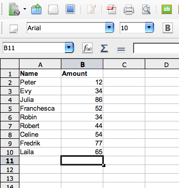
Create a list as shown here. Start with the headings in A1 and B1, and the data just below. It is good practice to always have a header in the columns, and keep the headers at the very first line of the spreadsheet, as it makes everything more tidy which, in turn, makes the table more predictable for formulas.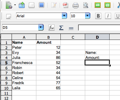
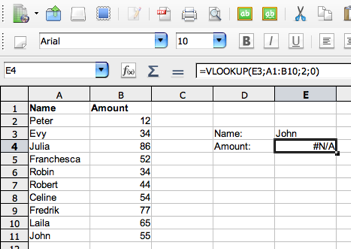
Go to cell D3 and enter "Name:". In D4 you enter "Amount:".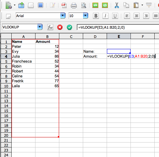
First we'll enter the formula and see the result, then we'll take a closer look at what's happening.
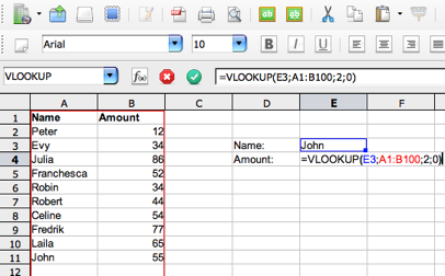
Go to E4 (the cell immediately to the right where you entered "Amount:", and enter: =VLOOKUP(E3;A1:B100;2;0)
NB! As you can see here, we're using a semi-kolon; ";", to separate inside the formula, your computer may be set up to use comma instead, ",". If so, correct the formula accordingly, everything else should be just the same.
OK, nothing interesting has happened so far, but you haven't done anything wrong! Now you can go to the next step.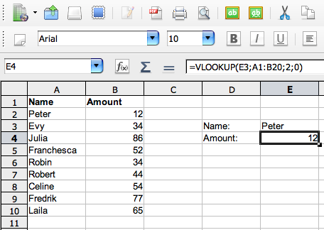
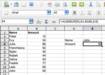
Now, go to E3 (the cell immediately to the right where you entered "Name:", and enter: "Peter". When you now press [Enter] you should see the number "12" in cell E4, where you typed the formula.
What happened here is that the formula tried to find the name you gave just above in the table to the left. If Calc finds the correct name, it's instructed to give you the corresponding amount.
Try experimenting with typing different names, also try entering wrong names, just to see what happens.
OK, now we'll start analyzing this formula. It looks ugly, but it really isn't that horrible once we get to break it up a bit.
Take another look at it: =VLOOKUP(E3;A1:B100;2;0)
Now we'll break it up: =VLOOKUP( what to search for ; where to search ; what result to give ; accuracy )
what to search for
This can either be a value or, as here, a cell reference. In our example we wanted to search for something related to "Peter", and we got that that value from cell E3. We would have excactly the same result if we replaced E3 with Peter, like this: =VLOOKUP("Peter";A1:B100;2;0)
where to search
This is the cell reference to the table we want to work with. In this case it is the area A1 to B100. As you see, the names are given in the left column, and the =VLOOKUP() formula will always search in the left column of any table. This is important.
The reason for typing B100, which is obviously too far down, is to make sure that if we add more data here, it will be included in the formula. Data enteret in cell A101 and B101 will not be considered by the formula. It is, by the way, not required that you include the column headings, like I’ve done here.
what result to give
If Calc is able to find what you wanted to search for, where you wanted to search for it, you need to specify exactly what information you want in return. In this case, we specified that we wanted the related information from column number 2 in the table. Notice that the number is totally unrelated to the cell reference itself -- of the same table was placed in the columns F and G, the reference number for the feedback would still be number 2, as it refers to the table you defined in the green area.
accuracy
OK, to be more accurate it really means sorted or not sorted... If it says "1", it means that the list is sorted, and will give you the closest match to what you searched for. You will probably never use that in you entire life, so I suggest that you consequently use "0" instead, which requires a perfect match. If it doesn't find a perfect match, it will show an error message: "#N/A".
You can also use the words "true" or "false" instead of, respectively, "1" or "0", with the exact same result -- but requires more typing! Sometimes less i more :-) Then it would look like this: =VLOOKUP(E3;A1:B100;2;false) Same - same, but more to type.
I hope that you now can see some of the potensial of this formula. Especially if you think BIG -- imagine having a huge list of 30 000 entries that you want to search! That is not unrealistic, I've done it houndreds of times myself.
As always, it is important to make sure that you lock the cell references by adding "$" to the cell references if you intend to copy the formula, for instance like this: =VLOOKUP($E$3;$A$1:$B$100;2;0) This way, if you copy the formula to the right, both the value you want to search for and the area in which you want to search will remain unchanged.
We will give you more examples of how to use =VLOOKUP() later.
A final advise; it is wise to define an area much longer than what you need at the moment to make sure that you can accommodate more lines of data (the green part of the formula). If you ad more data to your table, it will automatically be included in the area to search in the formula. If you use a limited area, you will need to update the formula manually.
First an example of what happens if you make it fit only the amount of data that you already have: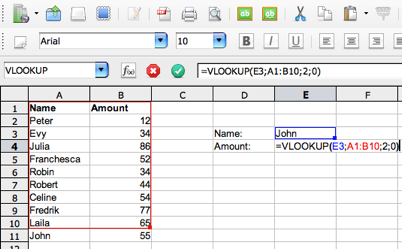
...then an example of what happens if you make it a bit wider: