< Previous lesson | Overview | Next lesson >
=SUMIF()
How to sum only lines meeting your criteria

=SUMIF() is one of those really powerful formulas, and is one that everybody who work with large lists should really get to know intimately.
With =SUMIF() you can sum all values in a column as long as the value on the same line in a different (or the same) column match a criteria you set.
Sounds complicated? Actually, it isn’t, believe it or not! Please go to the next step, and I’ll show how to use it.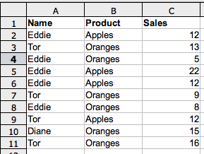
Imagine that you have a list with these columns:
- Column A: Name
- Column B: Product
- Column C: Sales
Now, to sum horisontally and vertically, we can use the excellent formula =SUM(), right? Right.
But it gets a bit more complicated the moment we want to sum only Eddies sales, doesn’t it? We could of course split sort each column and create one list for each person and use =SUM(). It would give you the correct amount, but it would involve a lot of work, and, in the end, the possibility of for errors will increase. Imagine the lists change all the time, and contains 10 000 lines...
This is where =SUMIF() can be an excellent solution!
What we’ll do, is to enter any name in a cell, and let Calc sum all values related to this name.
The syntax is: =SUMIF([Column to be evaluated];[Criteria];[Column to sum if criteria is met])
[Column to be evaluated]
In our example, this will be column A. So, in our example, if the name is "Eddie" is found in column A, it will be summed, otherwise it will be ignored.
[Criteria]
This is the criteria to be fulfilled in [Column to be evaluated]. This can be a formula, a value or a cell reference. In this case, it refers to cell F3, where Eddies name is.
[Column to sum if criteria is met]
If the criteria in the first column is met, this column is the one to sum. In our example, that would be the column for Sales, column C.
Please note that [Column to be evaluated] and [Column to sum if criteria is met] can actually be the same column! You could for instance specify that all values greater than 10 in column C should be summed.
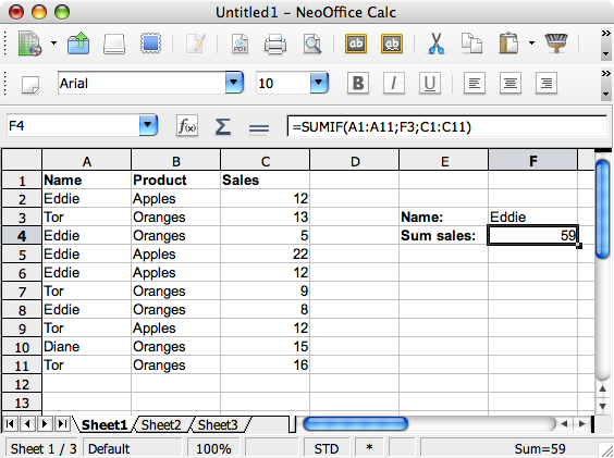
Here’s a nice colorization of the formula used in our example:
=SUMIF(A1:A11;F3;C1:C11)
You can now try to change the name between Eddie, Diane and Tor. Also, try to enter a name that’s not included in the list, just to see what happens.
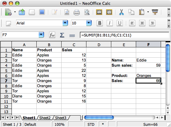
This time we’ll ad the ability to sum by product in the same manner.
Instead of having the [Column to be evaluated] to be column A, we’ll use column B, as you can see above.
Try entering Oranges, Apples and others, and see what happens!