< Previous lesson | Overview | Next lesson >
Sum it up
Our first, real formula...
The sum formula will be our first, real formula! This is one of the definitively most widely used formulas.
The formula is built like this: =sum()
I guess the point of the formula is quite obvious, to "sum" something... To be more specific, to sum any number of numbers. With the sum formula you can enter the numbers to sum or you can refer to cells in which the numbers are. We’ll excamplify the latter now.
OK, let’s jump right into it! Make a list of numbers like this:
Now we’ll try to sum these numbers, enter the formula as following: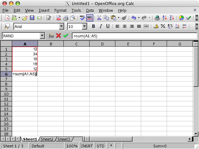
The "=" is very important, this tells OpenOffice that this is a formula. The word sum is important because it tells Calc what to do with the numbers. The paranthesis with the cell references are used to show Calc which numbers to do something with.
Now, here’s a really cool trick; start entering the forumula =sum( and nothing else! Now click on the topmost cell that contains the numbers, and hold the mouse button down while you drag down until you have marked the entire area you want to evaluate. Enter ), the ending paranthesis.
What happened now? Calc actually entered the cell adresses for you!
When you hit [Enter], your numbers will be summed, like this: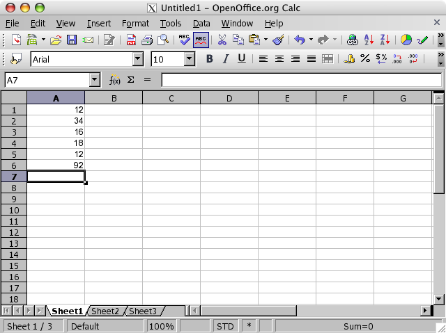
Now, try changing the uppmost value. Do that by clicking once on the cell, and start typing the number you want entered: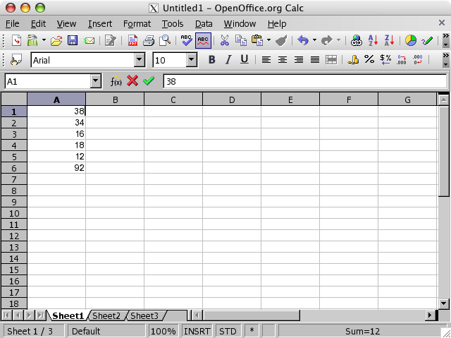
Now you’ll see that Calc automatically updates the sum to reflect the changes: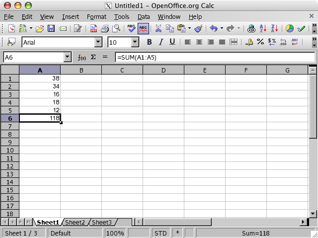
OK, delete the sum formula by selecting the cell, hit the [Delete] button, and finally [Enter]. Re-enter the same formula as before: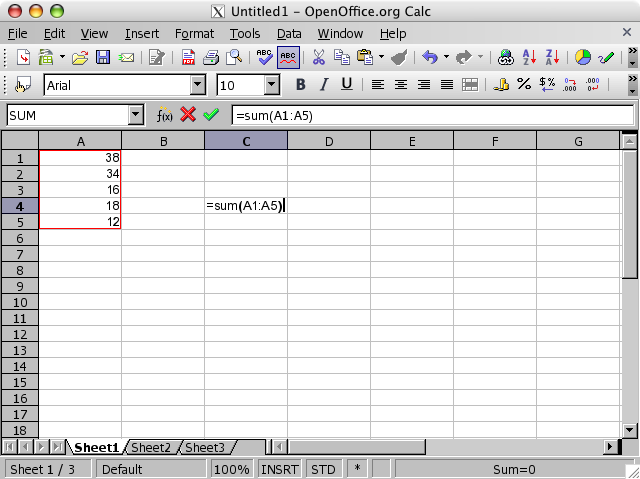
When you hit [Enter], you get the sum to the right of the area. This shows that you can place the sum wherever you want, which you will experience sooner or later is invaluable!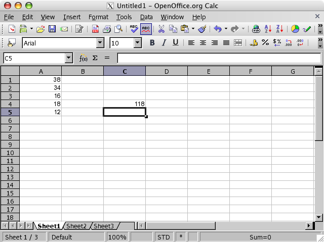
Now, try to enter a new number below the number in cell A5, like below: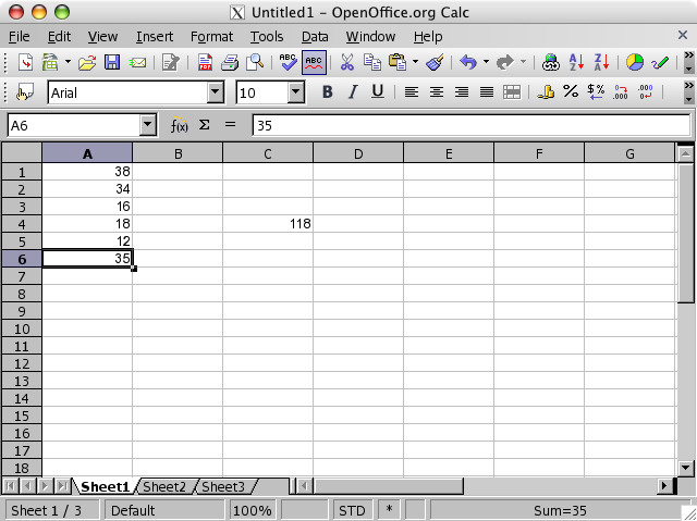
What happened with the sum formula? Nothing! Why? Because we didn’t allow the formula to include any new number. Go to the cell which contains the formula, press [F2] to enter the edit mode. The cells inclued in the formula will be bordered to show which area is included in the formula. At the bottom right of the formula you’ll see a handle, which you now should click and hold, and drag down, so that you include also the new number you entered: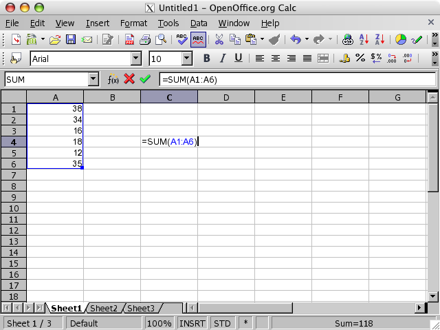
Hit [Enter], and see that the formula now includes the last number you entered.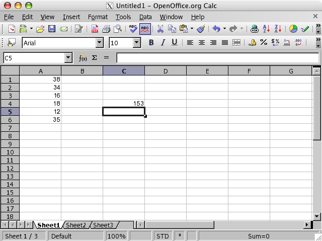
Again, go to the the formula and hit [F2].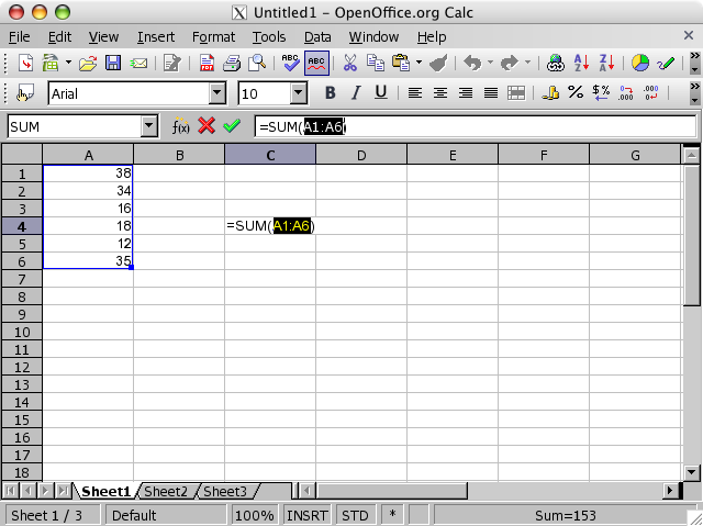
Change A6 to A1000: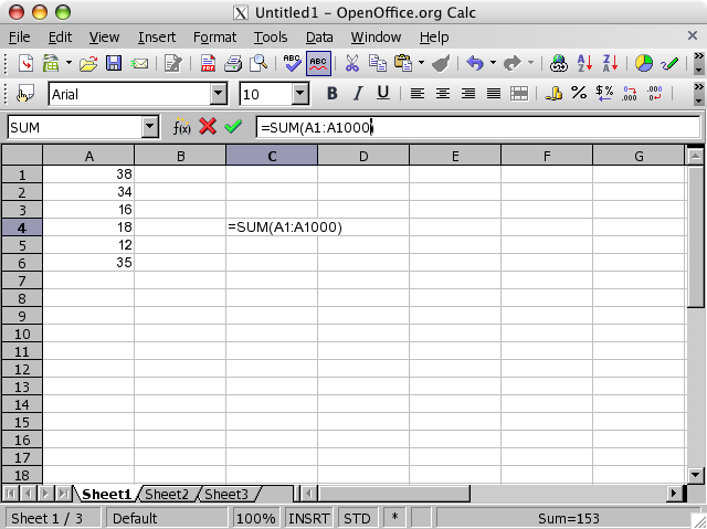
Now, try to enter new numbers below the others, and see what happens... You are now able to enter new numbers without having to update the formula each time! Well, until you’ve got 1000 numbers anyway... If you expect to reach that many numbers, you can increas the number from A1000 to A10000 e.g. But try it as you’ve edited now: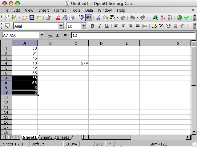
NB: The dark marking is done to examplify new numbers.